Advanced topics#
#
#
Multiple independent sublattices - from \(\text{TiN} \rightarrow \left(\text{Ti}_{0.25} \text{Al}_{0.25} \right) \left( \text{B}_{0.25} \text{N}_{0.25} \right)\)#
Now we want to enhance the above examples, and want to distribute both Ti and Al on the original Ti sublattice.
Furthermore, additionally, we want to distribute B and N on the original nitrogen sublattice. Before going into detail,
please download the example input files, the B2 structure
as well as the YAML input.
Before we start let’s investigate the coordination shells of the input structure
sqsgen compute shell-distances ti-al-b-n.yaml
[0.0, 2.126767, 3.0077027354075403, 3.6836684998608384, 4.253534, 4.755595584303295, 5.209493951789751, 6.015405470815081, 6.380301, 7.367336999721677]
we can interpret this number is the following way

Within the sphere of the first coordination shell (\(R_1 \approx 2.12\; \mathring A\)) of a Ti atom there are only N atoms. While versa holds true too, within the second coordination shell (\(R_2 \approx 3.08\; \mathring A\)) there are only atoms of the same type.
YAML file and the B2 structure# 1structure:
2 supercell: [2, 2, 2]
3 file: ti-n.cif
4iterations: 5e6
5shell_weights:
6 2: 1.0
7composition:
8 B:
9 N: 16
10 N:
11 N: 16
12 Ti:
13 Ti: 16
14 Al:
15 Ti: 16
The specification of the composition tag now differs from the previous examples
Line 6: Only consider second shell. Therefore, we automatically eliminate the Ti-B, Ti-N, Al-Ti and Al-V interactions
Line 8-11: Deals with the (original) N sublattice, you can interpret the input int the following way
Line 8-9: Distribute B atoms on the original N sublattice and put 16 of there
Line 10-11: Distribute N atoms on the original N sublattice and put 16 of there
Line 12-15: Deals with the (original) Ti sublattice, you can interpret the input int the following way
Line 12-13: Distribute Ti atoms on the original Ti sublattice and put 16 of there
Line 10-11: Distribute Al atoms on the original Ti sublattice and put 16 of there
Since in the example above we care only about the second coordination shell, we eliminate all interactions between the two sublattices. Let’s examine the output, therefore run the above example with
sqsgen run iteration --dump-include objective --dump-include parameters ti-al-b-n.yaml
Using those options will also store the Short-Range-Order parameters \(\alpha^i_{\xi\eta}\) and the value of the objective function \(\mathcal{O}(\sigma)\) in the resulting yaml file.
Those parameters should look something like this
objective: 5.4583
parameters:
- - [-0.0625, -0.875, 1.0, 1.0]
- [-0.875, -0.0625, 1.0, 1.0]
- [1.0, 1.0, -0.2083, -0.583]
- [1.0, 1.0, -0.583, -0.2083]
in the ti-al-b-n.result.yaml file.
The atomic species are in ascending order with respect to their ordinal number. For this example it is B, N, Al, Ti The above SRO parameters are arranged in the following way (see target_objective parameter).
We immediately see that the SRO is 1.0 if the constituting elements sit on different sublattices. This is because there are no pairs there \(N_{\xi\eta}^2 = 0\).
“Wrong” SRO parameters
Although the above example works and computes results, it does it not in a way we would expect it. Your can clearly observe this by \(\alpha_{\text{N-B}} < 0\) and \(\alpha_{\text{Al-Ti}} < 0\)
The SRO parameters are not wrong but mean something differently. We have restricted each of the species to only half of the lattice positions. In other words from the 64 initial positions Ti and Al are only free to choose 32 two of them (the former Ti sublattice).
Let’s consider Ti and Al for this particular example. According to Eq. (1) the SRO \(\alpha_{\text{Al-Ti}}\) is defined as
In the example above \(N=64\) and \(M^2=12\) while \(x_{\text{Al}} = x_{\text{Ti}}=\frac{1}{4}\) which leads to 48 expected Al-Ti pairs
However, Al and Ti are not allowed to occupy all \(N\) sites but only rather \(\frac{N}{2}\) (Same is also true for B and N) In addition the \(\frac{N}{2}\) sites, are allowed to be occupied only by Al and Ti, consequently we have to change \(x_{\text{Al}} = x_{\text{Ti}}=\frac{1}{2}\). This however leads to 96 expected bonds.
To fix this problem the above example need to be modified in the following way
YAML file and the B2 structure# 1structure:
2 supercell: [2, 2, 2]
3 file: ti-n.cif
4iterations: 5e6
5shell_weights:
6 2: 1.0
7composition:
8 B:
9 N: 16
10 N:
11 N: 16
12 Ti:
13 Ti: 16
14 Al:
15 Ti: 16
16prefactors: 0.5
17prefactor_mode: mul
Line 16: As the number of expected bonds changes, in the case of independent sublattices from 48 to 96. The “prefactors” \(f_{\xi\eta}^i\) (see Eq. (6)) represent the reciprocal value of the number of expected bonds and therefore need to be multiplied by \(\frac{1}{2}\) as \(\frac{1}{2}\cdot \frac{1}{48} \rightarrow \frac{1}{96}\)
Line 17: “mul” means that the default values of \(f_{\xi\eta}^i\) are multiplied with the values supplied from the prefactor parameters. \(\tilde{f}^i_{\xi\eta} = \frac{1}{2}f_{\xi\eta}^i\)
fine-tuning the optimization#
Note that although, the aforementioned SRO’s remain constant they contribute to the objective function \(\mathcal{O}(\sigma)\). One can avoid this by setting the pair-weights parameter (\(\tilde{p}_{\xi\eta}^i=0\) in Eq. (8)). Anyway the minimization will work.
We refine the above example in the following way
 1structure:
 2  supercell: [2, 2, 2]
 3  file: ti-n.cif
 4iterations: 5e6
 5shell_weights:
 6  2: 1.0
 7composition:
 8  B:
 9    N: 16
10  N:
11    N: 16
12  Ti:
13    Ti: 16
14  Al:
15    Ti: 16
16prefactor_mode: mul
17prefactors: 0.5
18pair_weights:
19 # B N Al Ti
20 - [ 0.0, 0.5, 0.0, 0.0 ] # B
21 - [ 0.5, 0.0, 0.0, 0.0 ] # N
22 - [ 0.0, 0.0, 0.0, 0.5 ] # Al
23 - [ 0.0, 0.0, 0.5, 0.0 ] # Ti
Line 18-23: set the pair-weight coefficients \(\tilde{p}_{\xi\eta}^i\).
The main diagonal is set to zero, meaning we do not include same species pairs
We set parameters of species on different sublattices (\(\alpha_{\text{B-Al}} = \alpha_{\text{N-Al}} = \alpha_{\text{B-Ti}} = \alpha_{\text{N-Ti}} = 0\)) to zero. This will result in a more “correct” value for the objective function
Note, that this modification has no influence on the SRO parameters itself, but only on the value of the objective function
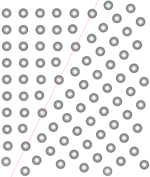
A \(\Sigma (210)[001]\) Ni grain boundary#
The following, example should illustrate how to use sqsgenerator for populating a structure which contains a planar defect. A symmetric tilt Ni
grain-boundary will serve as an example. The picture below shows a visual representation
of the grain-boundary. The red line represents the boundary plane.
To elucidate the difference between pure fcc Ni and the grain-boundary, we investigate the pair distribution function. Actually we create a histogram of the pair distance-matrix. For a perfect (fcc) crystal, the distance \(r_{ij}\) between two \(i\) and \(j\) can only approach discrete values. In the picture below this is shown by the red vertical lines. Thus, sqsgenerator will detect those values and use them as coordination shell parameter and consequently implicitly set sensible values to the shell_distances parameter.

The grain-boundary, however, breaks the symmetry and therefore the spikes smear out, as shown in the figure above.
Therefore, it is likely that sqsgenerator does not detect all or finds too many coordination shells. It is advisable
to set the coordination radii manually. An example input file for this special grain boundary
case is available. Nevertheless, the values computed by default should serve as a decent starting
guess. You can always print the computed default values by executing:
sqsgen compute shell-distances ni5.yaml
To set the shell distances manually we have to specify them in the input files. Therefore, one has to provide values for the coordination shell radii in \(\mathrm{\mathring{A}}\) using the shell_distances parameters.
1structure:
2  file: ni5.vasp
3shell_distances: [0.0, 2.7, 3.9, 4.65, 5.3, 5.8, 6.27, 6.8, 7.9, 8.49]
4composition:
5  Ni: 190
6  Al: 190
What happens under the hood is shown in the figure below.

The translucent green lines represent the “guesses” made by sgsgen’s internal routines. While it is decent for the first few shells, once the peaks get closer it misses some of them. The blue lines correspond to the values specified in the above example.
Moreover, sqsgenerator can plot the pair-distance histogram and will draw computed coordination-shell radii, similar to the graph shown above. Therefore, just draw the diagram using the –plot option. This will print the histogram as well as estimated and user-specified coordination shell radii.
sqsgen compute shell-distances --plot ni5.yaml
Non-integer values of \(M^i\)
In equation Eq. (3), \(M^i\) denotes the number of atoms in a coordination shell. Often \(M^i\) is also called the “coordination number. E. g. \(M^1 = 12\) for a fcc lattice. For perfect lattices this number will be an integer.
However, if not all atoms in the input cell exhibit the same amount of neighbors in the \(i^{\mathrm{th}}\) coordination shell, \(M^i\) will exhibit an non-integer value.
This might occur for example if the input structure …
exhibits a point or planar defect, as shown above
underwent ionic relaxtion before
However, for perfect lattices, which we assume as the “standard” use case, a non-integer value of \(M^i\) would be a problem. Therefore, sqsgenerator will print a warning, which should be ingored for the current example.
Optimal structure with unknown cell shape#
sqsgen itself only permutes configurations, and not cell shapes. Nevertheless, one can perform an optimization for different cell shapes individually. Therefore, we provide a function which allows to execute multiple optimization loops asynchronously.
To generate the supercell shapes, the following example relies on the ICET
package. We use icet.tools.enumerate_supercells,
which itself implements an algorithm to find such cell shapes\(^{1,2}\) which do not lead to symmetrically equivalent cells.
Therefore, to keep thins simple we try to find a supercell for \(\mathrm{Au}_{0.5}\mathrm{Pd}_{0.5}\). We search cell sizes containing 2-14 atoms with a step size of two. This ensures that each cell will have the desired composition
All we need to do is to write a function which generates input for sqsgen.
from ase.build import bulk
from collections import Counter
from icet.tools.structure_enumeration import enumerate_supercells
from sqsgenerator.public import from_ase_atoms, total_permutations

supercell_sizes = list(range(2, 15, 2))  # 2, 4, 6, ...
fcc_au = bulk('Au')

def make_sqsgen_input():
    # enumerate over all supercells and generate sqsgen input
    for supercell in enumerate_supercells(fcc_au, supercell_sizes):
        natoms = int(0.5 * len(supercell))  # distribute both natoms Au and Pd atoms
        atoms = from_ase_atoms(supercell).with_species(['Au'] * natoms + ['Pd'] * natoms)
        yield dict(
            structure=atoms,
            composition=Counter(atoms.symbols),
            mode='systematic',  # search all possible configurations
            similar=True,  # find all structures that minimize the objective function,
            max_output_configurations=total_permutations(atoms)  # use 1 if you want to find the best only
        )
Once we have defined such a function producing input, we can execute it directly, and let sqsgen merge the results for us. To actually execute the optimizations for each of the supercell-shapes we can use the following snippet.
from sqsgenerator.tools import sqsgen_minimize_multiple
best_objective, structures = sqsgen_minimize_multiple(generate_sqsgen_input())
print(f"Found {len(structures)} best structure with objective {best_objective}")
Note: As we have set max_output_configurations=total_permutations(atoms) in the first snippet, this example is
going to result in a lot of structures as it keeps all configuration. In case one needs to find only one best structure
set similar=False and omit the max_output_configurations in the first code listing.
\(^1\) G. L. W. Hart and R. W. Forcade, Algorithm for generating derivative structures, Physical Review B 77, 224115 (2008), 10.1103/PhysRevB.77.224115
\(^2\) G. L. W. Hart and R. W. Forcade, Generating derivative structures from multilattices: Algorithm and application to hcp alloys, Physical Review B 80, 014120 (2009), 10.1103/PhysRevB.80.014120